Useful concepts for critical appraisal: 3. association, outcomes and errors

Correlation

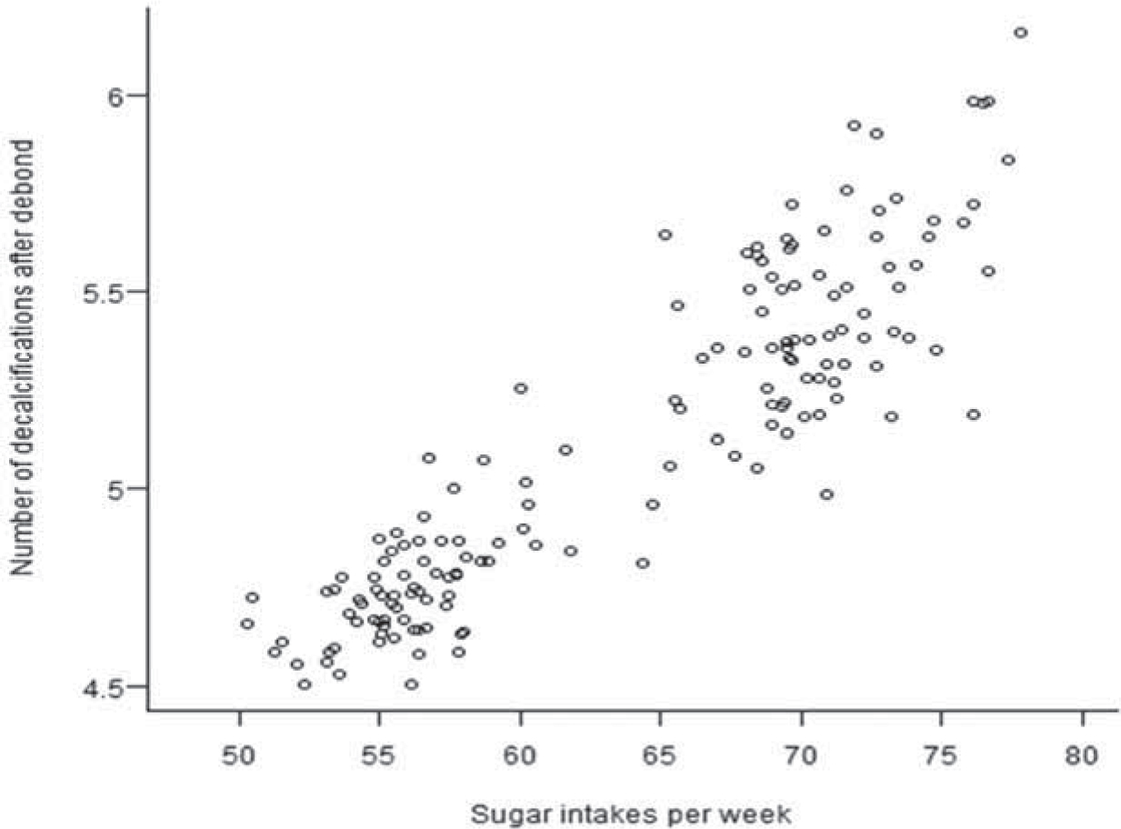
Correlation is concerned with the strength of linear association between two variables measured on the same individual. By convention, the variables are plotted on a scatterplot so that the independent (explanatory) variable is on the x-axis and the dependent (response) variable is on the y-axis (Figure 1).

Correlation coefficients

A correlation coefficient can be calculated to describe the magnitude and direction of any linear association, but it cannot suggest whether the relationship is causal. Hypothesis tests for correlation can be undertaken and a p-value may be displayed in the results: the null hypothesis presumes there is no linear association whatsoever. Both parametric and non-parametric versions of correlation coefficient exist:

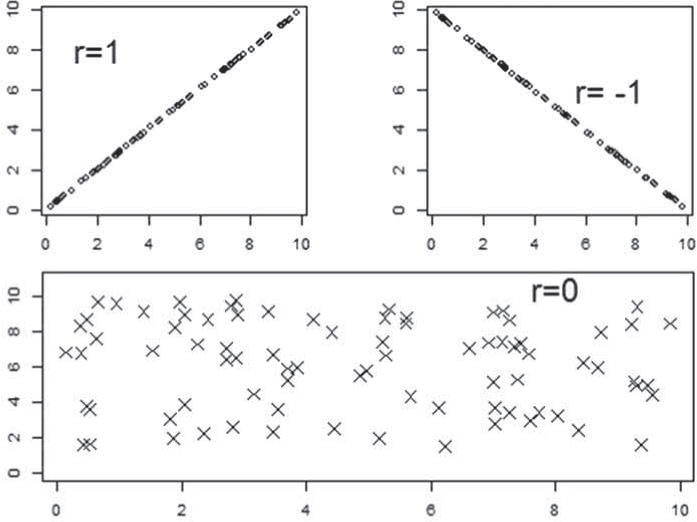
Pearson's correlation coefficient (parametric data): This is appropriate if the data are normally distributed with equal variance along the length of a line. The value in the population is estimated in the sample: known as ‘r’. It lies between +1 and -1 (Figure 2). The magnitude indicates how close the points are to the straight line (degree of scatter). The sign indicates if one variable increases as the other increases or decreases (as shown by positive or negative values). If r = 0 then there is no linear association. The ‘r²' value is often displayed in the results. This represents the proportion (%) of variability of y that can be attributed to its linear relationship with x.

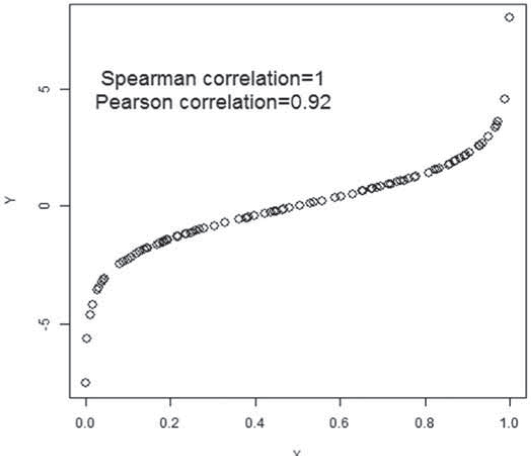
Spearman's rank (ρ) or Kendall's (τ) correlation coefficient (non-parametric data): If the data do not satisfy the requirements for a Pearson correlation to be valid then these are rank correlation coefficients (Figure 3) which give a measure of the tendency for one variable to rise (or fall) as the other increases (in any fashion, not necessarily linearly). Note that there is no equivalent of r².

Regression

Regression models can be used to describe the relationship between two or more variables: x (the independent variable/s) and y (the dependent variable) via an equation (Box 1).

The independent explanatory variables may be numeric, categoric or a mixture. The appropriate regression model to use depends on the type of the outcome variable:

Although analyses of variance (ANOVAs), Kruskal-Wallis tests and other extensions of the basic ANOVA can be used to investigate joint associations between several variables, regression analyses are preferable since they yield more useful information and are considered more flexible. Regression models can allow for non-uniform data structures and yield effect sizes (confidence intervals as well as p-values). Regression analyses also make it possible to examine the relationships between several independent (x) variables to make predictions about the outcome. They are used to measure the joint associations different variables may have on a study outcome and can be used to make adjustments for possible confounders.

Linear regression

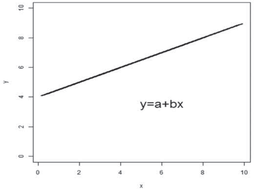
Simple linear regression is used when there is a single numeric dependent variable (y) and one independent explanatory variable (x). It involves estimating a best-straight line to summarize the association (Figure 4).

Residuals are the differences between the values predicted from the equation and the actual values. Small residuals would indicate a model that fits well.

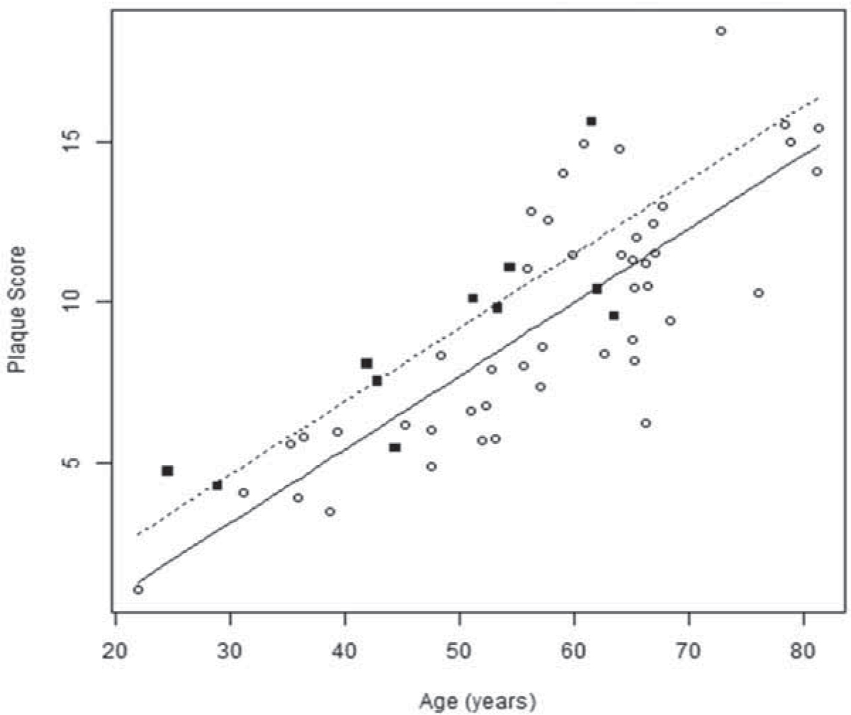
Multiple linear regression is used when there is one numeric dependent variable (y) but several independent explanatory variables (many xs). Extending the above concept, multiple regression allows one to examine the relationships between several variables and make predictions about the outcome. It is used to assess the joint associations variables may have on a study outcome and adjust for the effects of possible confounders. One measure of goodness of fit is given by an R² value which represents what proportion of the variability of y can be explained by its relationship with all of the xs in the model. Thus, for example, an R² of 0.4 means that only 40% of the variation in the dependent variable can be explained by the explanatory variables included in the model. Figure 5 provides an example of multiple linear regression.

Survival analysis

Survival analysis techniques are appropriate when the outcome is the time to an event occurring and that event has not yet occurred for all individuals in the dataset. For example, a study may investigate survival (non-debond) of orthodontic brackets in this way.

The brackets which have not reached the endpoint (debonded) by the end of the study (or during the time they were observed for) are described as censored. Because of the censored observations it is not possible to determine the mean survival time, so median values are used, but note that these can only be calculated if at least half have had the event by the end of follow-up.

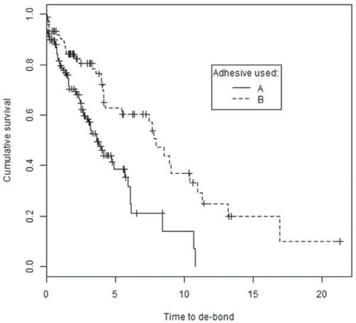
The data are often presented in Kaplan–Meier life tables and groups can be compared using survival curves. The life table and survival curves estimate the probability of a bracket ‘surviving’ (ie not debonding) at a given time after the start time (Figure 6).

A survival ‘curve’ is not smooth but reduces in steps each time an event occurs. Between the steps there may be many individuals who are censored. Symbols may be superimposed on the curve to indicate censored observations.

Median survival time is the time from the start of a study that coincides with a 50% probability of survival.

Log rank test

The survival experiences of two groups can be compared using the non-parametric log rank test. The null hypothesis assumes that there is no difference in survival experience between the two groups. For example, the above example, survival (non-debond) of brackets using two different bracket adhesives can be compared in this way.

One problem with the log-rank test is that it yields a p-value but not a measure of effect size (confidence interval).

Cox proportional hazards regression analysis

The hazard is the instantaneous probability of an individual reaching the endpoint in a study at a given time conditional upon survival up to that time. Regression models can be built with the logarithm of the hazard of the event occurring at any time as the outcome. Several independent or explanatory (x) variables may be incorporated into the models to measure the joint associations different variables have on a study outcome and/or to adjust for possible confounders.

The hazard ratio is a comparison of the hazard values between two groups, complemented by a p value and confidence intervals. If the hazard ratio is 1, then there is no increased or decreased risk. If it is >1, the factor increases the risk. If <1, the factor decreases the risk of the event at any given time. Proportional hazards are generally assumed, meaning that the relative hazard is the same at all time points. A Cox regression model fitted to the data in Figure 6 relating to bracket debonds using two different adhesives showed that the hazard of de-bonding was 1.839 times (95% CI 1.34, 2.52), p<0.0005, higher for those in group A.

Extending the above example, the explanatory variables in the regression analysis might be age, gender, income and literacy level.

Error studies

It is very important to acknowledge that any research may be subject to error. This can affect the reliability of the work and its interpretation. Note that errors can be both systematic (regular, indicating bias) or random.

Error studies for numerical variables

The Bland and Altman method² allows for both a simple estimate of agreement between two measurements of the same object (reliability) or between two methods (reproducibility). There are two parts (Box 2).

Box 2.

There are essentially two reasons for undertaking an error study:¹

Assessment of reproducibility: This assesses whether two techniques produce the same result or if two observers obtain the same results. It is the ability of a method to be accurately reproduced by someone else working independently. This is also known as the error of the method or as inter-examiner or inter-instrument error.

Assessment of repeatability: This assesses whether a single observer obtains the same results in repeated measurements. It is the variation in measurements taken by a single person or instrument under the same conditions − a measurement is said to be repeatable if the variation is smaller than some agreed limit. This is also known as the error of measurement or as intra-examiner or intra-instrument error.

Check for any bias. For this, there are two elements:

A paired t-test (for parametric data) or Wilcoxon signed ranks test (for non-parametric data) on the differences between the results.

A plot of the differences (y-axis) against the means of the first and second values (on the x-axis) – if there is random scatter around 0 then there is no bias. Systematic errors (bias) result in an offset of the points from this line and outliers represent random errors.

Measurement of agreement. Again, there are two elements:

The differences between the results are examined and the British Standards Institute repeatability coefficient is often calculated. This indicates the maximum difference likely to occur between the two measurements if there is no bias. This is calculated as 2 x estimated SDs of the differences.

The 95% limits of agreement give the range within which we can expect 95% of the differences in the population to lie between, assuming normality. These are calculated from the sample mean +/− BSI repeatability coefficients. This allows a visual assessment of the repeatability. Confidence intervals should also be calculated around the limits of agreement to show how precisely they are estimated (Figure 7).

Other methods associated with describing errors are listed in Box 3.

Box 3.

Other methods associated with describing errors:

Dahlberg's d³: This quantifies the precision of the measurements: in general, the smaller the calculated value, the more exact the measurement.

Intraclass correlation coefficient: This a measure of the extent to which paired (or serial) measurements from the same individual are more alike than values from different individuals. A value of 1 indicates perfect agreement.

Pearson's correlation coefficient: This does not assess agreement, only association. The value will be 1 if the points lie on any line.

References

Petrie A, Watson PFOxford: Wiley Blackwell; 2006
Bland JM, Altman DG Measuring agreement in method comparison studies. Stat Methods Med Research. 1999; 8:(2)135-160
Harris EF, Smith RN Accounting for measurement error: a critical but often overlooked process. Arch Oral Biol. 2009; 54:s107-s117